6. BSPM JMAG 2D FEA Analyzer

This analyzer enables the 2-D transient FEA evaluation of select bearingless surface permanent magnet machine topologies with DPNV windings in JMAG.

6.1. Model Background

Bearingless motors are electric machines capable of simultaneously creating both torque and forces. FEA tools are generally required to evaluate the performance capabilities of these machines. This analyzer does everything that is required for evaluating a BSPM design from drawing the machine geometry to solving the magnetic vector potential matrices. The code has been tested and confirmed to be compatible with JMAG v19 and above. The motor shaft and magnets are assumed to be conductive, and therefore, eddy current losses are enabled in these components. As there are several configurations that can be modified for any FEA evaluation, a JMAG_2D_Config is provided to work alongside this analyzer. A description of the configurations users have control over from within this class is provided below.

6.1.1. Time Step Size

A key enabling factor of FEA is that it discretizes machine evaluation both in time and in space. The control users have over time step size with this analyzer is elaborated below.

The BSPM FEA analyzer has been set up such that it has 2 distinct time steps. The underlying concept behind having 2 distinct time steps is to allow artificially created transient effects during FEA solver initialization to dampen out before using FEA data to evaluate the motor’s performance. Both time steps have 2 variables: number of revolutions and number of steps per revolution. Users should change these values based on what makes the most sense for their machine. Generally, the step size should be the same across both time steps, with the 1st time step running for a lesser number of revolutions. It is recommended that the 2nd time step should last for at least a half revolution to get reliable information on the motor’s performance capabilities.

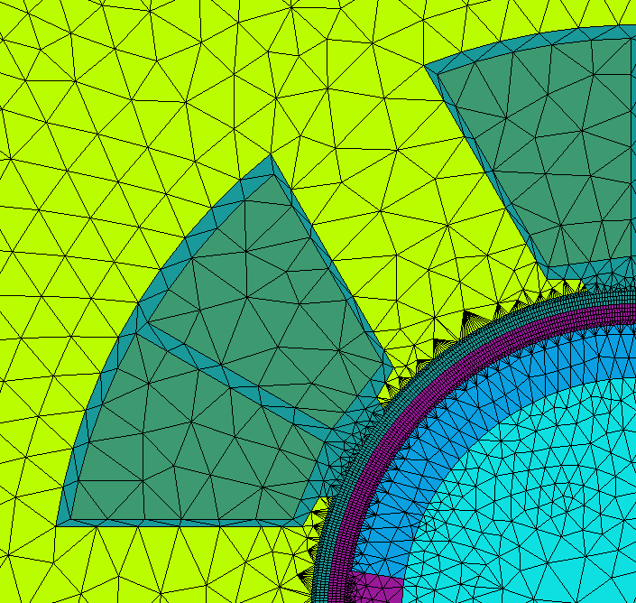
6.1.2. Mesh Size

Meshing is the method by which FEA tools discretize the motor geometry. In this analyzer, we use the slide mesh feature of JMAG. In addition to a generic mesh size setting for the model, separate handles are provided for the magnet and airgap meshes in the JMAG_2D_Config class. It is recommended that both the airgap and magnet mesh be significantly denser than that of other components for obtaining accurate results. Users should balance mesh density with result accuracy to get reliable results as quickly as possible. Figures showing the mesh layout of an example motor design are provided below.

6.1.3. Other Configurations

In addition to time step and mesh size, several other changes can be made to the BSPM JMAG analyzer. Most of these configurations are self explanatory and are described using comments within the JMAG_2D_Config class. For example, by setting the jmag_visible to True or False, users can control whether the JMAG application will be visible while a FEA evaluation is running. One can control the version of JMAG desired for use in this analyzer using jmag_version. For example, the use of JMAG-Designer21.1 would require an input of 21.1.

6.2. Input from User

To use the JMAG BSPM FEA analyzer, users must pass in a BSPM_EM_Problem object. An instance of the BSPM_EM_Problem class can be created by passing in a machine and an operating_point. The machine must be a BSPM_Machine and the operating_point must be of type BSPM_Machine_Oper_Pt. More information on both these classes is available here. The tables below provides the input expected by the BSPM_EM_Problem class and the input required to initialize the BSPM_EM_Analyzer

BSPM_EM_Problem Input

Arguments	Description
machine	object of type BSPM_machine describing a bearingless spm machine
operating_point	object of type BSPM_Machine_Oper_Pt describing BSPM machine operating point

BSPM_EM_Analyzer Initialization

Arguments	Description
config	object of type JMAG_2D_Config specifying time step, mesh settings, whether to model magnet/shaft eddy currents

Example code initializing both the analyzer and problem for the optimized BSPM design provided in this paper is shown below:

import numpy as np
from matplotlib import pyplot as plt
import os

from eMach.mach_eval.machines.materials.electric_steels import Arnon5
from eMach.mach_eval.machines.materials.jmag_library_magnets import N40H
from eMach.mach_eval.machines.materials.miscellaneous_materials import (
    CarbonFiber,
    Steel,
    Copper,
    Hub,
    Air,
)
from eMach.mach_eval.machines.bspm import BSPM_Machine
from eMach.mach_eval.machines.bspm.bspm_oper_pt import BSPM_Machine_Oper_Pt

from eMach.mach_eval.analyzers.electromagnetic.bspm.jmag_2d import (
    BSPM_EM_Problem,
    BSPM_EM_Analyzer,
)
from eMach.mach_eval.analyzers.electromagnetic.bspm.jmag_2d_config import JMAG_2D_Config

################ DEFINE BSPM machine ################
bspm_dimensions = {
'alpha_st': 44.5,
'd_so': 0.00542,
'w_st': 0.00909,
'd_st': 0.0169,
'd_sy': 0.0135,
'alpha_m': 178.78,
'd_m': 0.00371,
'd_mp': 0.00307,
'd_ri': 0.00489,
'alpha_so': 22.25,
'd_sp': 0.00813,
'r_si': 0.01416,
'alpha_ms': 178.78,
'd_ms': 0,
'r_sh': 0.00281,
'l_st': 0.0115,
'd_sl': 0.00067,
'delta_sl': 0.00011
}

bspm_parameters = {
'p': 1,
'ps': 2,
'n_m': 1,
'Q': 6,
'rated_speed': 16755.16,
'rated_power': 5500.0,
'rated_voltage': 240,
'rated_current': 10.0,
'name': "ECCE_2020",
}

bspm_materials = {
"air_mat": Air,
"rotor_iron_mat": Arnon5,
"stator_iron_mat": Arnon5,
"magnet_mat": N40H,
"rotor_sleeve_mat": CarbonFiber,
"coil_mat": Copper,
"shaft_mat": Steel,
"rotor_hub": Hub,
}

bspm_winding = {
"no_of_layers": 2,
"layer_phases": [ ['U', 'W', 'V', 'U', 'W', 'V'],
                    ['W', 'V', 'U', 'W', 'V', 'U'] ],
"layer_polarity": [ ['+', '-', '+', '-', '+', '-'],
                    ['-', '+', '-', '+', '-', '+'] ],
"coil_groups": ['b', 'a', 'b', 'a', 'b', 'a'],
"pitch": 2,
"Z_q": 49,
"Kov": 1.8,
"Kcu": 0.5,
"phase_current_offset": 0
}

ecce_2020_machine = BSPM_Machine(
        bspm_dimensions, bspm_parameters, bspm_materials, bspm_winding
    )

################ DEFINE BSPM operating point ################
ecce_2020_op_pt = BSPM_Machine_Oper_Pt(
            Id=0,
            Iq=0.975,
            Ix=0,
            Iy=0.025,
            speed=160000,
            ambient_temp=25,
            rotor_temp_rise=55,
            )

########################### DEFINE BSPM EM Problem ##########################
bspm_em_problem = BSPM_EM_Problem(ecce_2020_machine, ecce_2020_op_pt)

########################## DEFINE BSPM EM Analyzer ##########################
jmag_config = JMAG_2D_Config(
    no_of_rev_1TS=3,
    no_of_rev_2TS=0.5,
    no_of_steps_per_rev_1TS=8,
    no_of_steps_per_rev_2TS=64,
    mesh_size=4e-3,
    magnet_mesh_size=2e-3,
    airgap_mesh_radial_div=5,
    airgap_mesh_circum_div=720,
    mesh_air_region_scale=1.15,
    only_table_results=False,
    csv_results=(r"Torque;Force;FEMCoilFlux;LineCurrent;TerminalVoltage;JouleLoss;TotalDisplacementAngle;"
                "JouleLoss_IronLoss;IronLoss_IronLoss;HysteresisLoss_IronLoss"),
    del_results_after_calc=False,
    run_folder=os.path.abspath("") + "/run_data/",
    jmag_csv_folder=os.path.abspath("") + "/run_data/JMAG_csv/",
    max_nonlinear_iterations=50,
    multiple_cpus=True,
    num_cpus=4,
    jmag_scheduler=False,
    jmag_visible=True,
    jmag_visible=None,
)

em_analysis = BSPM_EM_Analyzer(jmag_config)

6.3. Output to User

The BSPM_EM_Analyzer returns a dictionary holding the results obtained from 2D FEA analysis of the machine. The elements of this dictionary and their description is provided below.

BSPM_EM_Analyzer Output

Output	Description
current	Data frame of coil currents vs time
voltage	Data frame of coil terminal voltage vs time
torque	Data frame of torque vs time
force	Data frame of force in x and y axes vs time
iron_loss	Data frame of iron loss at different frequencies
hysteresis_loss	Data frame of hysteresis loss at different frequencies
eddy_current_loss	Data frame of eddy current loss vs time
copper_loss	Analytically estimated copper loss
range_fine_step	Elements of dataframe over second time step

Example code using the analyzer to evaluate the example BSPM design and determine torque and force performance is provided below. The results are observed to closely match expected performance as provided in the paper.

########################## Solve design ##########################
results = em_analysis.analyze(bspm_em_problem)

############################ extract required info ###########################
from eMach.mach_eval.analyzers.force_vector_data import (
    ProcessForceDataProblem,
    ProcessForceDataAnalyzer,
)
from eMach.mach_eval.analyzers.torque_data import (
    ProcessTorqueDataProblem,
    ProcessTorqueDataAnalyzer,
)

length = results["current"].shape[0]
i = length - results["range_fine_step"]
results["current"] = results["current"].iloc[i:]

results["torque"] = results["torque"].iloc[i:]
results["force"] = results["force"].iloc[i:]
results["voltage"] = results["voltage"].iloc[i:]
results["hysteresis_loss"] = results["hysteresis_loss"]
results["iron_loss"] = results["iron_loss"]
results["eddy_current_loss"] = results["eddy_current_loss"].iloc[i:]

############################ post processing #################################
torque_prob = ProcessTorqueDataProblem(results["torque"]["TorCon"])
torque_analyzer = ProcessTorqueDataAnalyzer()
torque_avg, torque_ripple = torque_analyzer.analyze(torque_prob)

print("Average torque is ", torque_avg, " Nm")
print(
    "Torque density is ",
    torque_avg
    / (ecce_2020_machine.V_rfe + ecce_2020_machine.V_sh + ecce_2020_machine.V_rPM),
    " Nm/m3",
)
print("Average power is ", torque_avg * 160000 * np.pi / 30, " W")

force_prob = ProcessForceDataProblem(
    Fx=results["force"][r"ForCon:1st"],
    Fy=results["force"][r"ForCon:2nd"],
)
force_ana = ProcessForceDataAnalyzer()
f_x, f_y, force_avg, Em, Ea = force_ana.analyze(force_prob)

rotor_weight = (
    ecce_2020_machine.V_rfe * ecce_2020_machine.rotor_iron_mat["core_material_density"]
    + ecce_2020_machine.V_sh * ecce_2020_machine.shaft_mat["shaft_material_density"]
    + ecce_2020_machine.V_rPM * ecce_2020_machine.magnet_mat["magnet_material_density"]
)
FRW = force_avg / (rotor_weight * 9.8)

print("Average force is ", force_avg, " N")
print("Force per rotor weight is ", FRW, " pu")
print("Force error angle is ", Ea, " deg")